Root Finding - Python Notebook

Root finding refers to the process of finding solutions to equations of the form f(x) = 0. This is a fundamental problem in numerical analysis and has various applications in science and engineering.

# First let's import necessary libs
import matplotlib.pyplot as plt
import numpy as np
import math

# Our first function
def f(x):
  return x**2 - 2

# Let's plot the function
x = np.arange(0, 3, 0.1)
plt.plot(x, f(x), label='f(x) = x^2 - 2')

plt.axhline(0, color='red', linestyle='--')
plt.axvline(0, color='green', linestyle='--')

plt.xlabel('x')
plt.ylabel('f(x)')

plt.title('Plot of f(x) = x^2 - 2')
plt.grid()
plt.legend()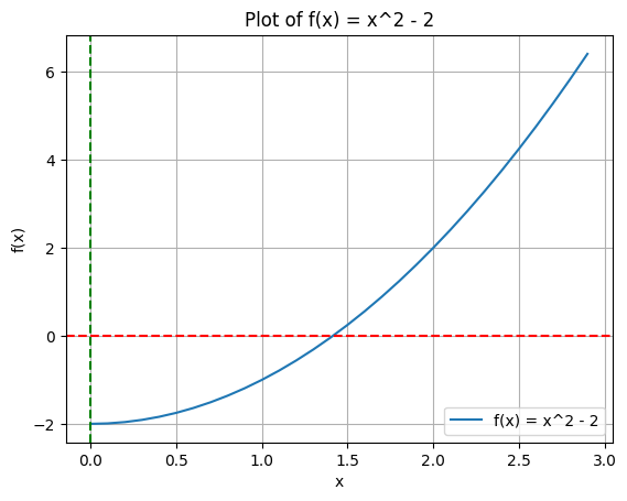

# Our second function
def f2(x):
  return x**3 - 4 * x + 1

# Let's plot the function
x = np.arange(-10, 10, 0.1)
plt.plot(x, f2(x), label='f2(x) = x^3 - 4x + 1')

plt.axhline(0, color='red', linestyle='--')
plt.axvline(0, color='green', linestyle='--')

plt.xlabel('x')
plt.ylabel('f2(x)')

plt.title('Plot of f2(x) = x^3 - 4x + 1')
plt.grid()
plt.legend()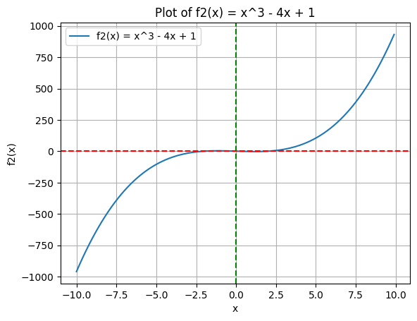

Bisection Method¶

Bisection method finds the root of a function f in the interval [a, b].

Parameters:
- f : function  
  The function for which we want to find the root.
- a : float  
  The start of the interval.
- b : float  
  The end of the interval.
- tol : float  
  The tolerance for convergence.

Returns:
- float  
  The approximate root of the function.

def bisection_method(f, a, b, tol=1e-5):
    if f(a) * f(b) >= 0:
        raise ValueError("f(a) and f(b) must have opposite signs.")

    mid = (a + b) / 2.0

    if abs(f(mid)) < tol:
        return mid
    elif f(a) * f(mid) < 0:
        return bisection_method(f, a, mid, tol)
    else:
        return bisection_method(f, mid, b, tol)

root = bisection_method(f, 0, 10)

# Let's plot the result
x = np.arange(0, 3, 0.1)

plt.plot(x, f(x), label='f(x) = x^2 - 2')
plt.scatter(root, f(root), color='blue')  # Mark the root on the plot
plt.axvline(root, color='purple', linestyle='--', label=f'x = root ({root:.5f})')

plt.axvline(0, color='green', linestyle='--')
plt.axhline(0, color='red', linestyle='--')

plt.xlabel('x')
plt.ylabel('f(x)')
plt.title(f"Bisection Method Root: {root:.5f}")
plt.grid()
plt.legend()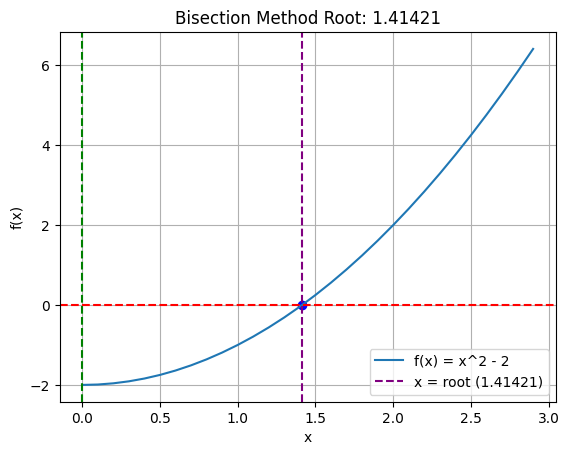

root = bisection_method(f2, -1, 1)

# Let's plot the result
x = np.arange(-10, 10, 0.1)

plt.plot(x, f2(x), label='f2(x) = x^3 - 4x + 1')
plt.scatter(root, f2(root), color='blue')  # Mark the root on the plot
plt.axvline(root, color='purple', linestyle='--', label=f'x = root ({root:.5f})')

plt.axvline(0, color='green', linestyle='--')
plt.axhline(0, color='red', linestyle='--')

plt.xlabel('x')
plt.ylabel('f2(x)')
plt.title(f"Bisection Method Root: {root:.5f}")
plt.grid()
plt.legend()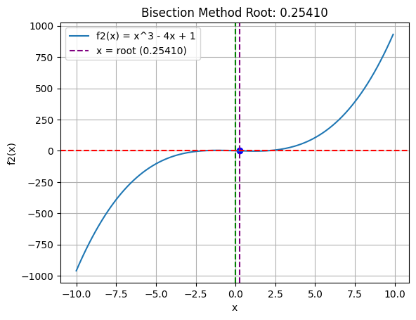

False Position Method¶

def false_position_method(f, a, b, tol=1e-5):
    if f(a) * f(b) >= 0:
        raise ValueError("f(a) and f(b) must have opposite signs.")

    c = a - (f(a) * (b - a)) / (f(b) - f(a))

    if abs(f(c)) < tol:
        return c
    elif f(a) * f(c) < 0:
        return false_position_method(f, a, c, tol)
    else:
        return false_position_method(f, c, b, tol)

root = false_position_method(f, 0, 10)

# Let's plot the result
x = np.arange(0, 3, 0.1)

plt.plot(x, f(x), label='f(x) = x^2 - 2')
plt.scatter(root, f(root), color='blue')  # Mark the root on the plot
plt.axvline(root, color='purple', linestyle='--', label=f'x = root ({root:.5f})')

plt.axvline(0, color='green', linestyle='--')
plt.axhline(0, color='red', linestyle='--')

plt.xlabel('x')
plt.ylabel('f(x)')
plt.title(f"False Position Method Root: {root:.5f}")
plt.grid()
plt.legend()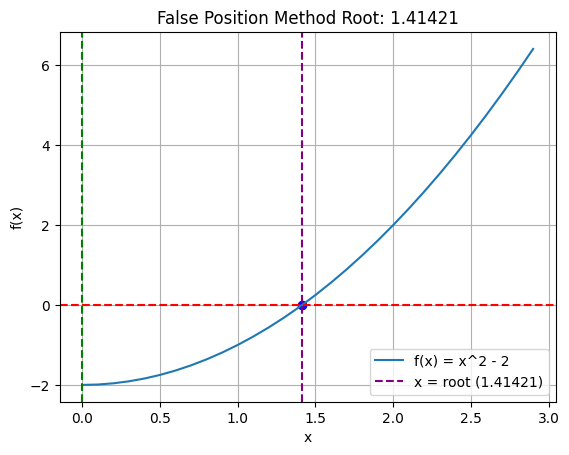

root = false_position_method(f2, -1, 1)

# Let's plot the result
x = np.arange(-10, 10, 0.1)

plt.plot(x, f2(x), label='f2(x) = x^3 - 4x + 1')
plt.scatter(root, f2(root), color='blue')  # Mark the root on the plot
plt.axvline(root, color='purple', linestyle='--', label=f'x = root ({root:.5f})')

plt.axvline(0, color='green', linestyle='--')
plt.axhline(0, color='red', linestyle='--')

plt.xlabel('x')
plt.ylabel('f2(x)')
plt.title(f"False Position Method Root: {root:.5f}")
plt.grid()
plt.legend()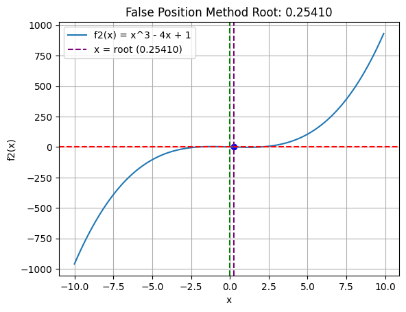

Iteration Method¶

The iteration method is a common approach to find roots of equations. It involves rearranging the equation into the form x = g(x) and then iteratively applying g to an initial guess until convergence.

Let’s consider the equation $x^3 - 4x + 1 = 0$ . We can rearrange it to $x = \frac{x^3 + 1}{4}$ .

def f2(x):
    return x**3 - 4*x + 1

def g2(x):
    return (x**3 + 1) / 4

Let’s implement the iteration methdod for this case,

def iteration_method(g, x, tol=1e-5, max_iter=100):
    for i in range(max_iter):
        x_new = g(x)
        if abs(x_new - x) < tol:
            return x_new
        x = x_new
    raise ValueError(
        "Iteration did not converge within the maximum number of iterations."
    )

And finally plotting time,

root = iteration_method(g2, 1)

# Let's plot the result
x = np.arange(-10, 10, 0.1)

plt.plot(x, f2(x), label='f2(x) = x^3 - 2x + 2')
plt.scatter(root, f2(root), color='blue')  # Mark the root on the plot
plt.axvline(root, color='purple', linestyle='--', label=f'x = root ({root:.5f})')

plt.axvline(0, color='green', linestyle='--')
plt.axhline(0, color='red', linestyle='--')

plt.xlabel('x')
plt.ylabel('f2(x)')
plt.title(f"Iteration Method Root: {root:.5f}")
plt.grid()
plt.legend()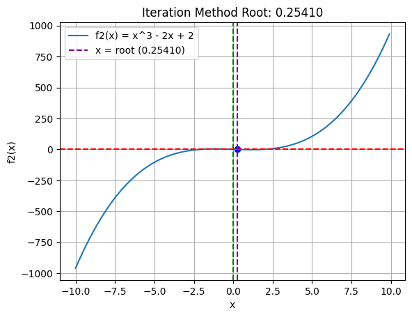

Newton-Raphson Method¶

The Newton-Raphson method is an efficient root-finding algorithm that uses the derivative of a function to find its roots. The method starts with an initial guess and iteratively refines it using the formula:

x_{n+1} = x_n - \frac{f(x_n)}{f'(x_n)}

(1)

where:

$x_n$ - is the current guess,
$f(x_n)$ - is the value of the function at $x_n$ ,
$f'(x_n)$ - is the value of the derivative of the function at $x_n$ .

# Our function
def f(x):
    return x**2 - 2

def df(x):
    return 2*x

# Newton-Raphson Method
def newton_raphson_method(f, df, x0, tol=1e-5, max_iter=100):
    x = x0
    for i in range(max_iter):
        x_new = x - f(x) / df(x)
        if abs(x_new - x) < tol:
            return x_new
        x = x_new
    raise ValueError(
        "Newton-Raphson method did not converge within the maximum number of iterations."
    )

root = newton_raphson_method(f, df, 1)
print(root)

1.4142135623746899

Let’s plot it...

root = newton_raphson_method(f, df, 10)

# Let's plot the result
x = np.arange(0, 3, 0.1)
plt.plot(x, f(x), label='f(x) = x^2 - 2')
plt.scatter(root, f(root), color='blue')  # Mark the root on the plot
plt.axvline(root, color='purple', linestyle='--', label=f'x = root ({root:.5f})')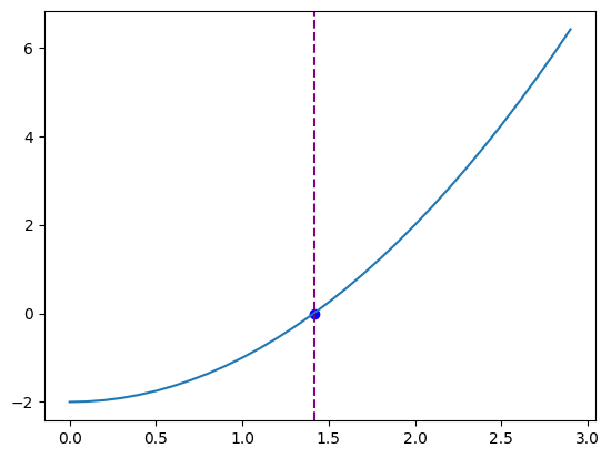

Secant Method¶

The secant method is a root-finding algorithm that uses two initial approximations to find the root of a function. Unlike the Newton-Raphson method, it does not require the computation of the derivative. Instead, it approximates the derivative using the two initial points.

The secant method uses the following formula to iteratively refine the root approximation:

x_{n+1} = x_n - f(x_n) \cdot \frac{x_n - x_{n-1}}{f(x_n) - f(x_{n-1})}

(2)

where:

$x_n$ is the current approximation,
$x_{n-1}$ is the previous approximation,
$f(x_n)$ is the value of the function at $x_n$ ,
$f(x_{n-1})$ is the value of the function at $x_{n-1}$ .

def secant_method(f, x0, x1, tol=1e-7, max_iter=100):
    for i in range(max_iter):
        if abs(f(x1)) < tol:
            return x1
        if f(x1) == f(x0):  # Prevent division by zero
            print("Division by zero encountered in secant method.")
            return None
        # Secant method formula
        x2 = x1 - f(x1) * (x1 - x0) / (f(x1) - f(x0))
        x0, x1 = x1, x2
    print("Maximum iterations reached without convergence.")
    return None

print(secant_method(f, 1, 2))

1.4142135620573204

Let’s plot it...

root = secant_method(f, 1, 2)

# Let's plot the result
x = np.arange(0, 3, 0.1)
plt.plot(x, f(x), label='f(x) = x^2 - 2')
plt.scatter(root, f(root), color='blue')  # Mark the root on the plot
plt.axvline(root, color='purple', linestyle='--', label=f'x = root ({root:.5f})')