Linear Regression - Python Notebook

In linear regression, we model the relationship between a dependent variable and one or more independent variables by fitting a linear equation to the observed data. The goal is to find the best-fitting line (or hyperplane in higher dimensions) that minimizes the difference between the predicted values and the actual values.

Let’s import the necessary libraries and create some sample data for linear regression.

import numpy as np
from sklearn.linear_model import LinearRegression
from matplotlib import pyplot as plt

Let’s create some sample data for linear regression. Let’s say we want to predict y from x using a linear relationship!

np.random.seed(0)
x = 2 * np.random.rand(100, 1)
y = 4 + 3 * x + np.random.randn(100, 1)

Create a linear regression model

model = LinearRegression()
model.fit(x, y)

Make predictions

x_new = np.array([[0], [2]])
y_predict = model.predict(x_new)

Print the coefficients

print("Intercept:", model.intercept_)
print("Coefficient:", model.coef_)

Intercept: [4.22215108]
Coefficient: [[2.96846751]]

Plot the results

plt.scatter(x, y)
plt.plot(x_new, y_predict, color='red')

plt.xlabel('X')
plt.ylabel('Y')

plt.title('Linear Regression')
plt.show()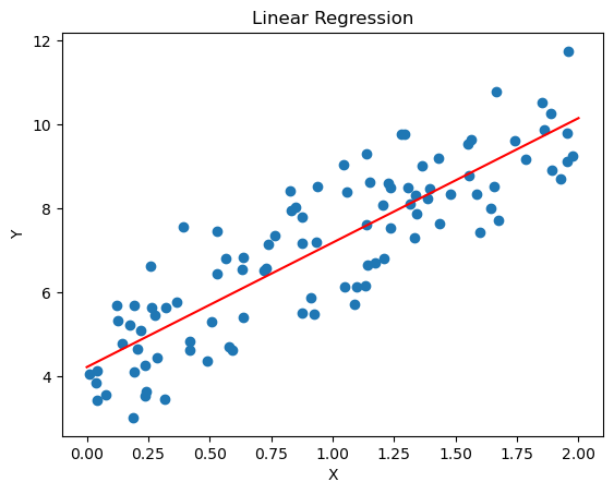

Gradient Descent¶

Gradient descent is an optimization algorithm used to minimize a function by iteratively moving towards the steepest descent, which is determined by the negative of the gradient. In the context of linear regression, gradient descent is used to find the optimal coefficients that minimize the cost function (usually the mean squared error).

def gradient_descent(x, y, m = 0, b = 0, learning_rate = 0.01, epochs = 10000):
    n = len(y)
    for _ in range(epochs):
        y_pred = m * x + b
        dm = (-2/n) * sum(x * (y - y_pred))
        db = (-2/n) * sum(y - y_pred)
        m -= learning_rate * dm
        b -= learning_rate * db
    return m, b

Let’s plot...

plt.scatter(x, y)

m, b = gradient_descent(x, y)
plt.plot(x, m*x + b, color='red')

plt.xlabel('X')
plt.ylabel('Y')

plt.title('Gradient Descent')
plt.show()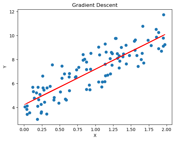

Stochastic Gradient Descent¶

Stochastic Gradient Descent (SGD) is a variant of the gradient descent algorithm that updates the model parameters using only a single or a few training examples at each iteration, rather than the entire dataset. This makes SGD more efficient for large datasets and can help the model converge faster.

def stochastic_gradient_descent(x, y, m=0, b=0, learning_rate=0.01, epochs=10000):
    n = len(y)
    for _ in range(epochs):
        for i in range(n):
            xi = x[i:i+1]
            yi = y[i:i+1]
            y_pred = m * xi + b
            dm = -2 * xi * (yi - y_pred)
            db = -2 * (yi - y_pred)
            m -= learning_rate * dm
            b -= learning_rate * db
    return m, b

Let’s plot it...

plt.scatter(x, y)

m, b = stochastic_gradient_descent(x, y)
plt.plot(x, m*x + b, color='red')

plt.xlabel('X')
plt.ylabel('Y')

plt.title('Stochastic Gradient Descent')
plt.show()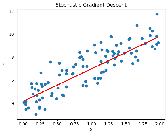

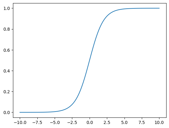
Logistic Regression (Bonus)¶

Logistic regression is a statistical method used for binary classification problems, where the goal is to predict the probability of an instance belonging to one of two classes. Unlike linear regression, which predicts continuous values, logistic regression predicts probabilities that are then mapped to discrete classes (0 or 1).

def logistic_regression(x):
    return 1 / (1 + np.exp(-x))

def predict_logistic(x, m, b):
    linear_combination = m * x + b
    return logistic_regression(linear_combination)

# An example usage
predict_logistic(0, 1, 0), predict_logistic(1, 1, 0), predict_logistic(-1, 1, 0)

(np.float64(0.5),
 np.float64(0.7310585786300049),
 np.float64(0.2689414213699951))

Let’s plot the curve...

x = np.linspace(-10, 10, 100)
y = logistic_regression(x)
plt.plot(x, y)