Logistic regression is used for binary classification tasks. It models the probability that a given input belongs to a particular class using the logistic function.
From Linear
Check the Linear Regression section’s last part.
From Polynomial
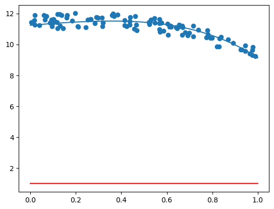
Let’s take the function from our previous polynomial regression example and convert it into a binary classification problem. We’ll classify points as belonging to class 1 if the output is greater than a certain threshold, and class 0 otherwise.
import numpy as np
import matplotlib.pyplot as plt

np.random.seed(0)
x = np.random.rand(100,1)
y = 3 * x**4 - 7 * x**3 + 2 * x**2 + 11 + np.random.rand(100,1)

# m0 x4 + m1 x3 + m2 x2 + m3 x + m4
def gd(x, y, m0=0, m1=0, m2=0, m3=0, m4=0, epoch=10000, learn=0.001):
    n = len(x)
    for i in range(epoch):
        y_n = m0 * x**4 + m1 * x**3 + m2 * x**2 + m3 * x + m4
        m4_l = - 2 / n * np.sum(y - y_n)
        m3_l = - 2 / n * np.sum((y - y_n) * x)
        m2_l = - 2 / n * np.sum((y - y_n) * x**2)
        m1_l = - 2 / n * np.sum((y - y_n) * x**3)
        m0_l = - 2 / n * np.sum((y - y_n) * x**4)

        m4 = m4 - learn * m4_l
        m3 = m3 - learn * m3_l
        m2 = m2 - learn * m2_l
        m1 = m1 - learn * m1_l
        m0 = m0 - learn * m0_l
    return m0, m1, m2, m3, m4

m0, m1, m2, m3, m4 = gd(x, y)
print(gd(x, y))
x_p = np.linspace(0, 1)

plt.plot(x_p, m0 * x_p**4 + m1 * x_p**3 + m2 * x_p**2 + m3 * x_p + m4)
plt.scatter(x,y)
(np.float64(-1.4008617749474424), np.float64(-1.237676294880945), np.float64(-0.689765797956417), np.float64(1.228140471950126), np.float64(11.237160966215388))
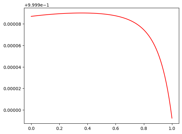
Let’s implement logistic based on the above function.
def logistic(z):
    return 1 / (1 + np.exp(-z))

def predict(x, m0, m1, m2, m3, m4, threshold=0.5):
    z = m0 * x**4 + m1 * x**3 + m2 * x**2 + m3 * x + m4
    return logistic(z)

x = np.linspace(0, 1, 100).reshape(-1, 1)
plt.plot(x, predict(x, m0, m1, m2, m3, m4), color='red')