Differential Equations - Python Notebook

A differential equation is a mathematical equation that relates a function with its derivatives. In simpler terms, it describes how a quantity changes in relation to another quantity. Differential equations are fundamental in various fields such as physics, engineering, and economics, as they model dynamic systems and processes.

Euler’s Method¶

Euler’s method is a simple and widely used numerical technique for solving ordinary differential equations (ODEs) with a given initial value. It is particularly useful for approximating solutions to first-order ODEs of the form:

\frac{dy}{dx} = f(x, y)

(1)

with an initial condition $y(x_0) = y_0$ .

Let’s consider an example,

\frac{dy}{dx} = x + y

(2)

y(0) = 1

(3)

Let’s import libraries first,

import numpy as np
import matplotlib.pyplot as plt

Our differential equation,

\frac{dy}{dx} = x + y

(4)

def f(x, y):
    return x + y

And our euler function,

def euler_method(f, x0, y0, h=0.1, n=100):
    x_values = [x0]
    y_values = [y0]
    
    for i in range(n):
        y0 = y0 + h * f(x0, y0)
        x0 = x0 + h
        x_values.append(x0)
        y_values.append(y0)
    
    return np.array(x_values), np.array(y_values)

Let’s plot and visualize the results,

# Initial conditions and parameters
x0 = 0
y0 = 1
h = 0.1  # Step size
n = 100  # Number of steps
x_values, y_values = euler_method(f, x0, y0, h, n)

# Plotting the results
plt.plot(x_values, y_values, label="Euler's Method", color='blue')
plt.title("Euler's Method for Solving ODE")
plt.xlabel('x')
plt.ylabel('y')
plt.legend()
plt.grid()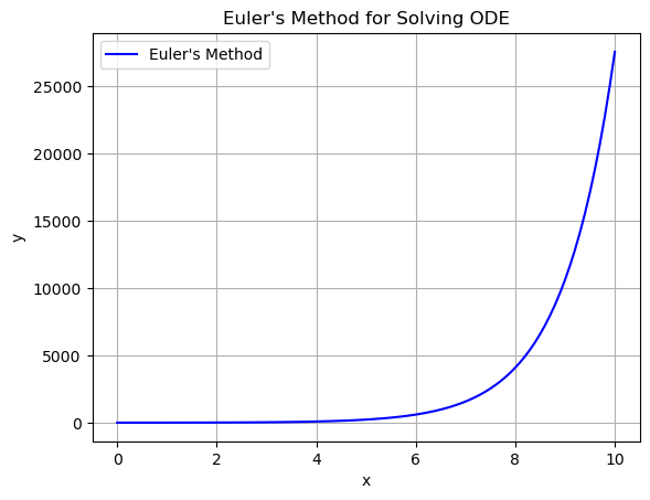

Runge-Kutta Method¶

The Runge-Kutta methods are a family of iterative methods used to solve ordinary differential equations (ODEs). The most commonly used version is the fourth-order Runge-Kutta method (RK4), which provides a good balance between accuracy and computational efficiency.

def runge_kutta_4th_order(f, y0, x0, x1, h):
    """
    y0: Initial value of y at x0
    x0: Initial value of x
    x1: Final value of x
    h: Step size
    f: Function that returns dy/dt given t and y
    """
    n = int((x1 - x0) / h)
    x_values = np.linspace(x0, x1, n + 1)
    y_values = np.zeros(n + 1)
    y_values[0] = y0

    for i in range(n):
        x = x_values[i]
        y = y_values[i]
        
        k1 = h * f(x, y)
        k2 = h * f(x + h / 2, y + k1 / 2)
        k3 = h * f(x + h / 2, y + k2 / 2)
        k4 = h * f(x + h, y + k3)
        
        y_values[i + 1] = y + (k1 + 2 * k2 + 2 * k3 + k4) / 6

    return x_values, y_values

Let’s plot it,

# Initial conditions and parameters for RK4
y0 = 1
x0 = 0
x1 = 10
h = 0.1
x_values, y_values_rk4 = runge_kutta_4th_order(f, y0, x0, x1, h)

# Plotting the results of RK4
plt.plot(x_values, y_values_rk4, label="Runge-Kutta 4th Order", color='red')
plt.title("Runge-Kutta 4th Order Method for Solving ODE")
plt.xlabel('t')
plt.ylabel('y')
plt.legend()
plt.grid()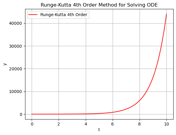

Picard’s Method¶

Picard’s method is an iterative technique used to approximate the solutions of ordinary differential equations (ODEs). It is particularly useful for solving initial value problems of the form:

\frac{dy}{dx} = f(x, y)

(5)

with an initial condition $y(x_0) = y_0$ .

Mathematically, Picard’s method constructs a sequence of functions that converge to the solution of the differential equation. The iterative formula is given by:

y_{n+1}(x) = y_0 + \int_{x_0}^{x} f(t, y_n(t)) \, dt

(6)

where $y_n(x)$ is the nth approximation of the solution.

So, first apporximation is,

y_1(x) = y_0 + \int_{x_0}^{x} f(t, y_0) \, dt

(7)

The second approximation is,

y_2(x) = y_0 + \int_{x_0}^{x} f(t, y_1(t)) \, dt

(8)

And so on...

For example, consider the initial value problem:

\frac{dy}{dx} = 1 + xy

(9)

y(0) = 1

(10)

# Apporoximations
def Y1(x):
    return 1 + (x) + pow(x, 2) / 2


def Y2(x):
    return 1 + (x) + pow(x, 2) / 2 + pow(x, 3) / 3 + pow(x, 4) / 8


def Y3(x):
    return (
        1
        + (x)
        + pow(x, 2) / 2
        + pow(x, 3) / 3
        + pow(x, 4) / 8
        + pow(x, 5) / 15
        + pow(x, 6) / 48
    )


def picard_method(f, x0, h=0.1, n=10, iterations=3):
    x_values = np.arange(x0, x0 + n * h, h)
    y_values = np.array([f(i) for i in x_values])

    return x_values, y_values

picard_method(f=Y3, x0=0, h=0.1)

(array([0. , 0.1, 0.2, 0.3, 0.4, 0.5, 0.6, 0.7, 0.8, 0.9]),
 array([1.        , 1.10534652, 1.22288933, 1.35518969, 1.50530133,
        1.67688802, 1.874356  , 2.10300152, 2.36917333, 2.68045019]))

Let’s plot it...

x_values, y_values = picard_method(f=Y3, x0=0, h=0.1)

plt.plot(x_values, y_values)
plt.scatter(x_values[1], y_values[1], label=f'Point at x={x_values[1]:.1f}')
plt.scatter(x_values[2], y_values[2], label=f'Point at x={x_values[2]:.1f}')
plt.legend()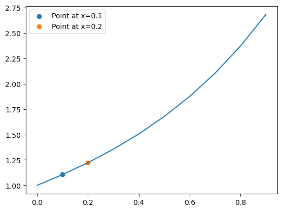

Milne’s Predictor-Corrector Method¶

Milne’s predictor-corrector method is a numerical technique used to solve ordinary differential equations (ODEs). It is a multi-step method that combines both prediction and correction steps to improve the accuracy of the solution.

The formula is,

y_{n+1, p} = y_{n-3} + \frac{4h}{3} \left( 2f_{n} - f_{n-1} + 2f_{n-2} \right)

(11)

y_{n+1} = y_{n-1} + \frac{h}{3} \left( f_{n+1, p} + 4f_{n} + f_{n-1} \right)

(12)

Where $y_{n+1, p}$ is the predicted value and $y_{n+1}$ is the corrected value.

If the value of n = 3, then our formula becomes,

y_{4, p} = y_{0} + \frac{4h}{3} \left( 2f_{3} - f_{2} + 2f_{1} \right)

(13)

y_{4} = y_{2} + \frac{h}{3} \left( f_{4, p} + 4f_{3} + f_{2} \right)

(14)

# Let's get x0, y0, x1, y1, x2, y2, x3, y3 from the picard method
x0, y0 = x_values[0], y_values[0]
x1, y1 = x_values[1], y_values[1]
x2, y2 = x_values[2], y_values[2]
x3, y3 = x_values[3], y_values[3]

print(f"x0: {x0}, y0: {y0}")
print(f"x1: {x1}, y1: {y1}")
print(f"x2: {x2}, y2: {y2}")
print(f"x3: {x3}, y3: {y3}")

# Let's get y4 from milne's method
def milne_method(x0, y0, x1, y1, x2, y2, x3, y3, x4, h=x1-x0):
    # Predictor
    y4_pred = y0 + (4 * h / 3) * (2 * f(x3, y3) - f(x2, y2) + 2 * f(x1, y1))
    # Corrector
    y4_corr = y2 + (h / 3) * (f(x2, y2) + 4 * f(x3, y3) + f(x4, y4_pred))
    return y4_corr

y4_milne = milne_method(x0, y0, x1, y1, x2, y2, x3, y3, x4=x3 + (x1 - x0))
print(f"y4 from Milne's method: {y4_milne}")

x0: 0.0, y0: 1.0
x1: 0.1, y1: 1.1053465208333333
x2: 0.2, y2: 1.2228893333333333
x3: 0.30000000000000004, y3: 1.3551896875
y4 from Milne's method: 1.5567806387037035