Numerical methods - viva

Basics: Numerical Methods

Errors & Core Concepts

1. Significant Figures: Determine by all non-zero digits, zeros between them, and trailing zeros if a decimal point is present. Leading zeros are not significant.

2. Accuracy vs. Precision: Accuracy is closeness to the true value. Precision is closeness of multiple measurements to each other (reproducibility).

3. Error Definitions: Round-off (from finite computer precision), Truncation (from approximating a method, e.g., cutting a Taylor series), and Formulation (from an imperfect model).

4. Round-Off Errors: Occur because computers use a finite number of bits. Mitigate with higher precision (e.g., double) or by reordering calculations to avoid subtracting nearly equal numbers.

5. Truncation Errors & Taylor Series: The Taylor series represents a function as an infinite sum of its derivatives. Truncation error comes from cutting off (truncating) this series after a finite number of terms.

6. Error Propagation: Errors in initial values accumulate through calculations. Estimated using formulas based on partial derivatives (propagation of uncertainty).

7. Total Numerical Errors: Total Error $\approx$ Truncation Error + Round-off Error. These two are often a trade-off (e.g., smaller step size $h$ reduces truncation but increases round-off).

8. Formulation Errors: Errors from using a simplified or flawed mathematical model to represent a real-world problem (e.g., ignoring friction).

9. Data Uncertainty: Handled with statistical methods (like Monte Carlo analysis) or interval arithmetic. It reduces the confidence and accuracy of the solution.

10. Error Analysis: Assessing reliability by analyzing the method’s truncation error (e.g., its order $O(h^p)$) and the potential for round-off error.

Here are additional viva questions and answers covering classification metrics.

Classification Metrics

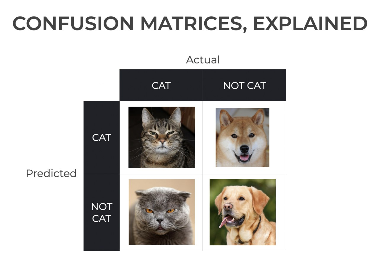
• What is a confusion matrix?

  A table that summarizes the performance of a classification model. It shows the counts of correct and incorrect predictions, broken down by their actual and predicted classes.

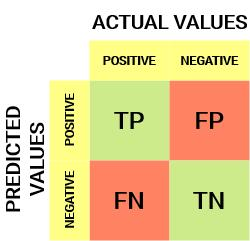
• Define True Positive (TP).

  TP: The model correctly predicted the positive class. (Actual: Positive, Predicted: Positive).

• Define True Negative (TN).

  TN: The model correctly predicted the negative class. (Actual: Negative, Predicted: Negative).

• Define False Positive (FP). What type of error is this?

  FP: The model incorrectly predicted the positive class when it was actually negative. (Actual: Negative, Predicted: Positive). This is a Type I Error.

• Define False Negative (FN). What type of error is this?

  FN: The model incorrectly predicted the negative class when it was actually positive. (Actual: Positive, Predicted: Negative). This is a Type II Error.

• How do you calculate Accuracy?

  Accuracy is the ratio of all correct predictions to the total number of predictions.

  • Formula: $(TP+TN)/(TP+TN+FP+FN)$

• What is Precision? What is its formula?

  Precision answers the question: “Of all the times the model predicted positive, how many were actually positive?” It measures a model’s “exactness.”

  • Formula: $TP/(TP+FP)$

• What is Recall (or Sensitivity)? What is its formula?

  Recall answers the question: “Of all the actual positive cases, how many did the model correctly identify?” It measures a model’s “completeness.”

  • Formula: $TP/(TP+FN)$

• What is Specificity? What is its formula?

  Specificity answers the question: “Of all the actual negative cases, how many did the model correctly identify?” It’s the “True Negative Rate.”

  • Formula: $TN/(TN+FP)$

• What is the F1-Score? Why is it useful?

  The F1-Score is the harmonic mean of Precision and Recall. It’s useful because it provides a single score that balances both Precision and Recall, which is especially important for imbalanced datasets where accuracy can be misleading.

  • Formula: $2\cdot (Precision\cdot Recall)/(Precision+Recall)$

• Give an example of a high-Precision, low-Recall scenario.

  A very cautious spam filter. It only marks emails as spam if it’s 100% sure (High Precision), but it lets some obvious spam get into your inbox (Low Recall).

• Give an example of a high-Recall, low-Precision scenario.

  A medical screening test for a dangerous disease. It’s designed to catch everyone who might have the disease (High Recall), but it also flags many healthy people for further testing (Low Precision).

• When would you prefer Precision over Recall?

  When False Positives (Type I Error) are more costly than False Negatives.

  • Example: Spam filtering. You would rather let some spam in (FN) than send an important email to the spam folder (FP).

• When would you prefer Recall over Precision?

  When False Negatives (Type II Error) are more costly than False Positives.

  • Example: Cancer detection. You would rather tell a healthy person they might be sick (FP) than tell a sick person they are healthy (FN).

---

Root Finding

General

• Transcendental equation? An equation containing non-algebraic functions (trigonometric, exponential, log). E.g., $e^x-\sin (x)=0$.

• Algebraic vs. Transcendental? Algebraic equations involve only polynomial expressions ($x^2+2x=0$). Transcendental equations involve functions like $\sin (x)$, $e^x$, $\log (x)$.

• Converge? The method’s approximations get closer and closer to the true root with each iteration.

• Order of convergence? How fast the method converges. Higher order = faster convergence.

Iteration Method (Fixed-Point Iteration)

• Principle? Rewrite $f(x)=0$ as $x=g(x)$ and iterate $x_{n+1}=g(x_n)$ until $x_n$ converges.

• Rewriting $f(x)=0$? No, the form $x=g(x)$ is not unique. (e.g., $x^2-x-2=0$ can be $x=\sqrt{x+2}$ or $x=x^2-2$).

• Condition for convergence? The absolute value of the derivative of $g(x)$, $|g^{\prime }(x)|$, must be less than 1 in the interval containing the root.

• Order of convergence? Linear (Order 1).

Bisection Method

• Principle? Repeatedly bisecting (halving) an interval and selecting the sub-interval in which the root must lie.

• Condition? The function $f(x)$ must be continuous, and the initial interval $[a,b]$ must satisfy $f(a)\cdot f(b)<0$ (i.e., $f(a)$ and $f(b)$ have opposite signs).

• Guaranteed to converge? Yes, always, if the initial conditions are met.

• Order of convergence? Linear (Order 1). It’s slow because it halves the interval (error) at each step.

• Iterations for accuracy $ϵ$? $n>\frac{\log ((b-a)/ϵ)}{\log (2)}$.

False Position Method (Regula Falsi)

• Improvement? It uses a secant line (a chord) to connect $(a,f(a))$ and $(b,f(b))$ instead of just taking the midpoint. The root approximation is where this line crosses the x-axis.

• Formula? $x_2=a-\frac{f(a)\cdot (b-a)}{f(b)-f(a)}$ (or $x_2=\frac{a\cdot f(b)-b\cdot f(a)}{f(b)-f(a)}$).

• Interval update? Same as bisection: keep the sub-interval where the sign of $f(x)$ changes.

• Convergence rate? Generally faster than bisection (superlinear).

• Drawback? One of the interval endpoints can get “stuck,” leading to slow convergence in some cases (e.g., for convex functions).

Newton-Raphson Method

• Geometric interpretation? Uses the tangent line to the curve at the current guess ($x_n$) to find the next guess ($x_{n+1}$) where the tangent hits the x-axis.

• Iterative formula? $x_{n+1}=x_n-\frac{f(x_n)}{f^{\prime }(x_n)}$. Derived from the first-order Taylor expansion.

• Info needed? The function $f(x)$, its derivative $f^{\prime }(x)$, and an initial guess $x_0$.

• Order of convergence? Quadratic (Order 2), which is very fast.

• Convergence conditions? The initial guess must be “sufficiently close” to the root, and $f^{\prime }(x)\ne 0$ near the root.

• When does it fail? If $f^{\prime }(x_n)=0$ (horizontal tangent), if the initial guess is poor (can diverge), or if it enters a loop.

Comparisons

• Bisection vs. False Position: Bisection is guaranteed but slow. False Position is usually faster but can be slow if one endpoint gets stuck.

• Bisection vs. N-R: Bisection is slow and reliable, only needs $f(x)$. N-R is very fast (quadratic) but requires $f^{\prime }(x)$ and a good initial guess, and can fail.

• Why N-R preferred? Its quadratic convergence (speed) is highly desirable, especially for complex problems where high precision is needed quickly.

---

Equation Solving

General

• System of linear equations? A set of two or more linear equations with the same set of variables.

• Direct vs. Iterative? Direct methods (like Gauss) find the exact solution in a finite number of steps (ignoring round-off error). Iterative methods start with a guess and refine it until it’s “close enough.”

• Which methods? Cramer’s, Gauss Elimination, and Gauss-Jordan are direct methods.

• Ill-conditioned system? A system where a small change in the coefficients or constant terms results in a large change in the solution.

Cramer’s Rule

• Principle? Uses determinants to solve a system $AX=B$.

• Finding $x_i$? $x_i=\frac{\det (A_i)}{\det (A)}$, where $A_i$ is the matrix $A$ with its $i$-th column replaced by the constant vector $B$.

• Disadvantage? Computationally very expensive (calculating many determinants) and inefficient for systems larger than 3x3.

• When not applicable? If the determinant of the coefficient matrix $A$ is zero ($\det (A)=0$), as this means the system has either no solution or infinitely many solutions.

Gauss Elimination Method

• Two steps? 1. Forward Elimination (reducing to upper triangular form). 2. Back Substitution (solving for variables from bottom to top).

• Forward elimination? Using elementary row operations to create zeros below the main diagonal, turning the matrix into an upper triangular form.

• Back substitution? Solving the last equation (which has only one variable), then substituting that value into the second-to-last equation, and so on, moving up.

• Pivoting? Swapping rows (partial pivoting) or rows and columns (full pivoting) to place the largest possible element in the pivot position. This is done to improve numerical stability and avoid division by zero or small numbers.

• Zero pivot? If a zero appears on the diagonal and cannot be removed by row-swapping with a row below it, the system does not have a unique solution.

Gauss-Jordan Elimination

• Difference? It continues the elimination process to create zeros above the main diagonal as well, resulting in a diagonal or identity matrix.

• Final form? The augmented matrix $[A|B]$ is reduced to $[I|S]$, where $I$ is the identity matrix and $S$ is the solution vector.

• Advantage? It directly gives the solution vector; no back-substitution is needed.

• Disadvantage? Requires more computations (approx. 50% more) than Gauss Elimination.

• Finding inverse? Augment the matrix $A$ with the identity matrix $[A|I]$ and reduce $A$ to $I$. The result will be $[I|A^{-1}]$.

---

Value Estimation (Interpolation)

General

• Interpolation? Estimating the value of a function between known data points.

• Interpolation vs. Extrapolation? Interpolation is estimating within the range of known data. Extrapolation is estimating outside that range (which is less reliable).

• Interpolating polynomial? A polynomial that passes exactly through all the given data points.

• Finite difference table? A table showing the differences between function values, and the differences of those differences, and so on.

Interpolation — Diagonal & Horizontal Differences

• Forward difference $\Delta$? $\Delta y_i=y_{i+1}-y_i$.

• Backward difference $\nabla$? $\nabla y_i=y_i-y_{i-1}$.

• Central difference $\delta$? $\delta y_i=y_{i+1/2}-y_{i-1/2}$.

• Forward difference table? A table listing $x$, $y$, $\Delta y$, ${\Delta }^{2}y$, etc. Used for Newton’s forward formula.

• Newton’s Forward? When interpolating near the beginning of a set of equally spaced data points.

• Newton’s Backward? When interpolating near the end of a set of equally spaced data points.

• Limitation? The data points ($x$ values) must be equally spaced.

Lagrange Interpolation Method

• Advantage? It can be used when the data points ($x$ values) are not equally spaced.

• Form? A sum of terms: $P(x)={\sum }_{i=0}^n{y}_i\cdot L_i(x)$.

• Basis polynomials $L_i(x)$? $L_i(x)$ is a polynomial designed to be 1 at $x=x_i$ and 0 at all other data points $x=x_j$ (where $j\ne i$).

• Disadvantage? If a new data point is added, the entire polynomial must be recalculated from scratch.

---

Integration Approximation (Numerical Integration)

General

• Why? To find the definite integral of a function that is too complex to integrate analytically (by hand) or when the function is only known as a set of data points.

• Newton-Cotes? A family of formulas (like Trapezoidal, Simpson’s) that approximate the integral by fitting a polynomial to the data points and integrating that polynomial.

Trapezoidal Rule

• Idea? Approximate the area under the curve $f(x)$ using a trapezoid (i.e., approximating $f(x)$ with a 1st-degree polynomial/straight line).

• Single-application formula? ${\int }_a^{b}f(x)dx\approx \frac{h}{2}[f(a)+f(b)]$, where $h=b-a$.

• Composite formula? ${\int }_a^{b}f(x)dx\approx \frac{h}{2}[y_0+2(y_1+y_2+...+y_{n-1})+y_n]$.

• Error order? Proportional to $h^2$.

Simpson’s 1/3 Rule

• Function? Approximates $f(x)$ using a quadratic polynomial (a parabola).

• Points/Intervals? Requires 3 points, which means 2 sub-intervals (or any even number $n$ of sub-intervals for composite).

• Composite formula? ${\int }_a^{b}f(x)dx\approx \frac{h}{3}[y_0+4(y_1+y_3+...)+2(y_2+y_4+...)+y_n]$.

• Error order? Proportional to $h^4$, which is much more accurate than Trapezoidal.

• Condition on $n$? $n$ (the number of sub-intervals) must be even.

Simpson’s 3/8 Rule

• Function? Approximates $f(x)$ using a cubic polynomial.

• Condition on $n$? $n$ (the number of sub-intervals) must be a multiple of 3.

• When preferred? When $n$ is a multiple of 3, or sometimes used in combination with the 1/3 rule if $n$ is odd.

• Accuracy? Also has an error order proportional to $h^4$, but is generally slightly less accurate (larger error constant) than the 1/3 rule.

---

Ordinary Differential Equations (ODE)

General

• Initial Value Problem (IVP)? An ODE where all required conditions (like $y(x_0)=y_0$) are specified at the same, single starting value of $x$.

• Single-step vs. Multi-step? Single-step methods (like Euler, RK4) find $y_{i+1}$ using only information from the previous step $y_i$. Multi-step methods (like Milne) use information from several previous steps ($y_i,y_{i-1},...$).

• Which methods? Single-step: Euler’s, Picard’s, Runge-Kutta. Multi-step: Milne’s.

Euler’s Method

• Interpretation? Takes the slope at the current point ($x_i,y_i$) and follows a straight line (the tangent) over a step $h$ to estimate the next point $y_{i+1}$.

• Formula? $y_{i+1}=y_i+h\cdot f(x_i,y_i)$.

• Error? Local error is $O(h^2)$ (error per step). Global error is $O(h)$ (total accumulated error).

• Why inaccurate? It’s a first-order method and assumes the slope is constant over the whole step $h$, which leads to large errors unless $h$ is extremely small.

Picard’s Method

• What is it? An iterative method that solves the ODE $y^{\prime }=f(x,y)$ by successively integrating it.

• How? It turns the ODE into an integral equation $y(x)=y_0+{\int }_{x_0}^{x}f(t,y(t))dt$ and iterates: $y_{n+1}=y_0+{\int }_{x_0}^{x}f(t,y_n(t))dt$.

• Drawback? The integration step can become very difficult or impossible to perform analytically after a few iterations.

Runge-Kutta (R-K) Methods

• Purpose? To get higher accuracy (like a Taylor series) without needing to calculate higher derivatives of $f(x,y)$.

• RK4? “4th order” means its global error is $O(h^4)$, which is very accurate.

• Idea of RK4? It calculates a weighted average of four slopes at different points within the interval $[x_i,x_{i+1}]$ (at the

  beginning, two in the middle, one at the end) to get a better estimate of the “true” slope over the interval.

• Why popular? It’s a single-step method, easy to implement, self-starting, and provides a very good balance of accuracy and computational effort.

• Single/Multi-step? It is a single-step method.

Milne’s Method (Milne-Simpson Predictor-Corrector)

• Predictor-Corrector? A multi-step method that first “predicts” a value for $y_{i+1}$ (using an explicit formula) and then “corrects” that prediction (using an implicit formula) to get a more accurate value.

• Formulas?

  • Predictor (Milne): $y_{i+1,P}=y_{i-3}+\frac{4h}{3}[2f_i-f_{i-1}+2f_{i-2}]$

  • Corrector (Simpson): $y_{i+1,C}=y_{i-1}+\frac{h}{3}[f_{i+1,P}+4f_i+f_{i-1}]$

• Why multi-step? The formulas depend on values from previous steps ($y_i,y_{i-1},y_{i-2},y_{i-3}$).

• How to start? You need 4 starting points. These are usually generated using a single-step method like RK4.

• Issue? Can suffer from numerical instability for certain types of ODEs.

---

Regression

General

• Regression? A statistical method to find a function (model) that best fits a set of data points, used for predicting trends or values.

• Interpolation vs. Regression? Interpolation must pass through all points. Regression finds a “best-fit” line/curve that minimizes the overall error and does not necessarily pass through any point.

• Residual? The vertical distance between an actual data point ($y_i$) and the value predicted by the regression model (${\hat{y}}_i$). Residual = $y_i-{\hat{y}}_i$.

Least Squares Regression

• Principle? Find the parameters (coefficients) of the model that minimize the sum of the squares of the residuals.

• Minimizing what? $\sum (y_i-{\hat{y}}_i{)}^2$.

• How to find parameters? Take the partial derivatives of the sum-of-squares error with respect to each parameter, set them to zero, and solve the resulting system of “normal equations.”

Linear Regression

• Model? $y=a_0+a_{1}x$, where $a_0$ is the y-intercept and $a_1$ is the slope.

• Normal equations? A 2x2 system for $a_0$ and $a_1$:

  • $\sum y_i=n\cdot a_0+a_1\cdot \sum x_i$

  • $\sum x_i{y}_i=a_0\cdot \sum x_i+a_1\cdot \sum x_i^2$

• $R^2$? The “coefficient of determination.” It measures what proportion of the variance in the dependent variable ($y$) is predictable from the independent variable ($x$). A value of 1.0 means a perfect fit.

Polynomial Regression

• Model? $y=a_0+a_{1}x+a_2{x}^2+...+a_m{x}^m$ (an $m$-th degree polynomial).

• Still “linear”? It’s “linear” because the model is linear in its coefficients ($a_0,a_1,...$). We are still solving a linear system of normal equations for these coefficients.

• Overfitting? Using too high of a polynomial degree, which makes the model fit the noise in the data perfectly but fail to generalize to new data. The curve will “wiggle” aggressively to hit all the points.

Logistic Regression

• When used? For classification problems, where the output $y$ is a discrete category (e.g., Yes/No, 0/1, Spam/Not Spam), not a continuous value.

• Sigmoid function? $g(z)=\frac{1}{1+e^{-z}}$. It “squashes” any real-valued input $z$ into an output between 0 and 1, which can be interpreted as a probability.

• What’s regressed? It finds a linear relationship for the log-odds (or “logit”) of the event: $\log (\frac{P}{1-P})={\beta }_0+{\beta }_{1}x$.

Stochastic Gradient Descent (SGD)

• Gradient Descent? An iterative optimization algorithm used to find the minimum of a cost function (like the sum-of-squares error). It “descends” by taking steps in the direction of the steepest negative gradient.

• Cost function? The function we want to minimize (e.g., Mean Squared Error in linear regression).

• Batch vs. Stochastic?

  • Batch GD: Calculates the gradient using the entire dataset in one go to update the parameters.

  • Stochastic GD (SGD): Calculates the gradient and updates the parameters using only one data point (or a small “mini-batch”) at a time.

• Epoch? One complete pass through the entire training dataset.

• Learning rate? A hyperparameter ($\alpha$) that controls how big of a step to take in the direction of the gradient.

  • Too large: Can overshoot the minimum and diverge.

  • Too small: Will take a very long time to converge.

• Advantage of SGD? It’s much faster per-update and can escape local minima, making it ideal for very large datasets.