Mastering Matplotlib! - Python Notebook

import matplotlib.pyplot as plt

Line Plots¶

plt.plot()

[]

plt.plot([2,4,6,8])

plt.plot([2,4,2,6,8,4])

salaries=[55000,65000,72000,90000,115000,150000]
ages = [20,25,30,32,40,45]
plt.plot(ages, salaries)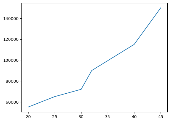

plt.plot(ages, salaries)
plt.show()

import numpy as np
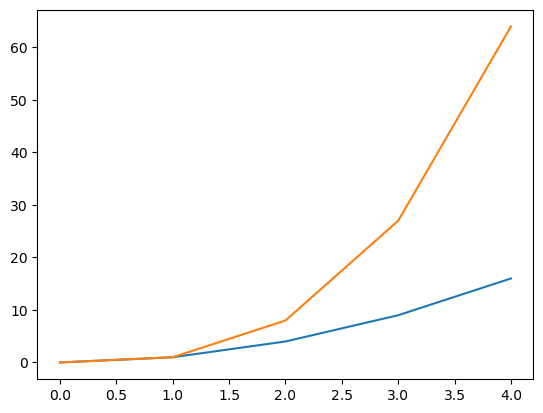
nums = np.arange(5)
nums

array([0, 1, 2, 3, 4])

plt.plot(nums,nums)
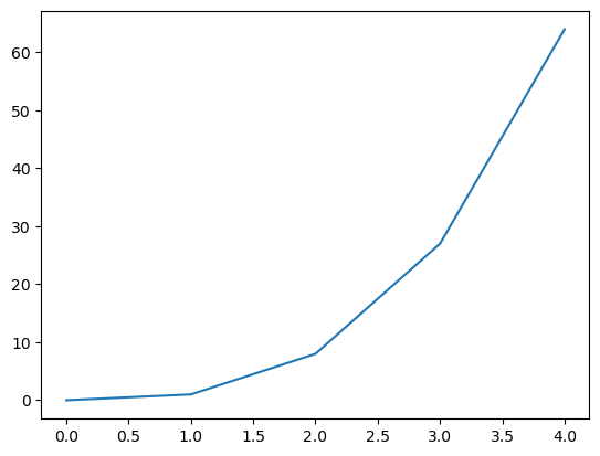
plt.plot(nums, nums*nums)
plt.plot(nums, nums**3)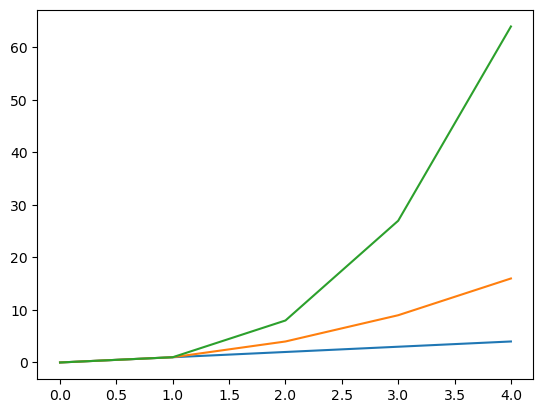

plt.figure()
plt.plot(nums,nums)
plt.figure()
plt.plot(nums, nums*nums)
plt.plot(nums, nums**3)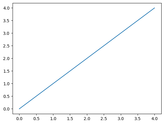

plt.figure()
plt.plot(nums,nums)
plt.figure()
plt.plot(nums, nums*nums)
plt.figure()
plt.plot(nums, nums**3)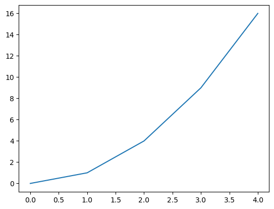

figsize¶

plt.figure(figsize=(2,6))
plt.plot(nums,nums)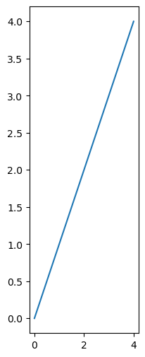

plt.figure(figsize=(6,6))
plt.plot(nums,nums**3)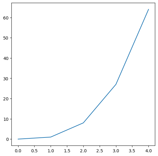

Plot styles¶

plt.style.available

['Solarize_Light2',
 '_classic_test_patch',
 '_mpl-gallery',
 '_mpl-gallery-nogrid',
 'bmh',
 'classic',
 'dark_background',
 'fast',
 'fivethirtyeight',
 'ggplot',
 'grayscale',
 'petroff10',
 'seaborn-v0_8',
 'seaborn-v0_8-bright',
 'seaborn-v0_8-colorblind',
 'seaborn-v0_8-dark',
 'seaborn-v0_8-dark-palette',
 'seaborn-v0_8-darkgrid',
 'seaborn-v0_8-deep',
 'seaborn-v0_8-muted',
 'seaborn-v0_8-notebook',
 'seaborn-v0_8-paper',
 'seaborn-v0_8-pastel',
 'seaborn-v0_8-poster',
 'seaborn-v0_8-talk',
 'seaborn-v0_8-ticks',
 'seaborn-v0_8-white',
 'seaborn-v0_8-whitegrid',
 'tableau-colorblind10']

plt.style.use('fivethirtyeight')

plt.plot(nums,nums)
plt.plot(nums, nums*nums)
plt.plot(nums, nums**3)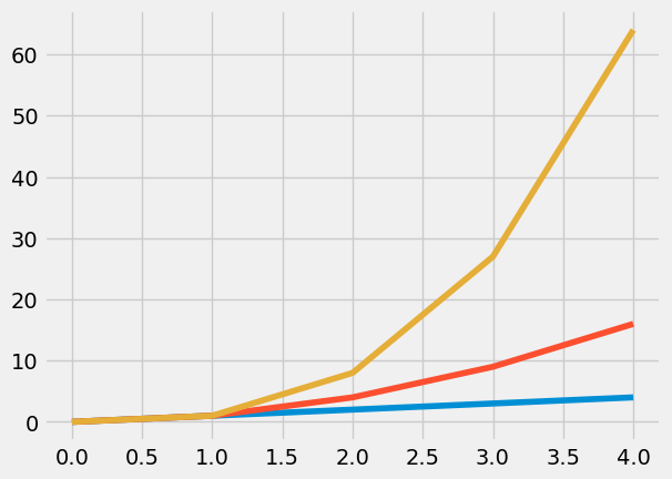

plt.style.use('dark_background')

plt.plot(nums,nums)
plt.plot(nums, nums*nums)
plt.plot(nums, nums**3)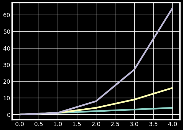

plt.style.use('ggplot')

plt.plot(nums, nums)
plt.plot(nums, nums*nums)
plt.plot(nums, nums**3)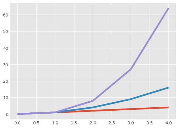

plt.style.use('default')

plt.plot(nums, nums, color="olive", linewidth=4)
plt.plot(nums, nums*nums, color="#ff6b6b", linewidth=4)
plt.plot(nums, nums**3, c="#ff9f43", linewidth=4)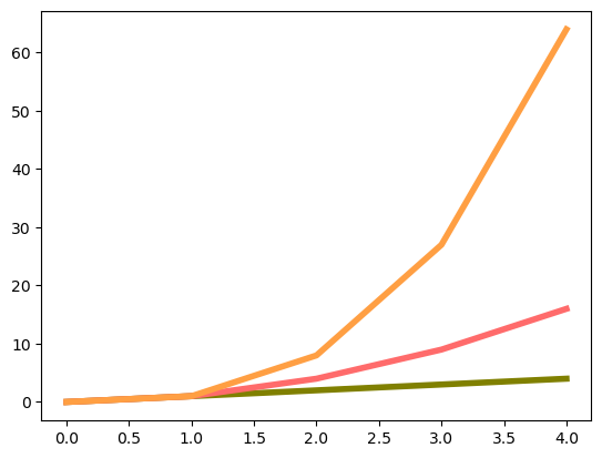

plt.plot(nums, nums, color="olive", linewidth=4, linestyle="dashed")
plt.plot(nums, nums*nums, color="#ff6b6b", linewidth=4, linestyle="dotted")
plt.plot(nums, nums**3, c="#ff9f43", linewidth=4, linestyle="-.")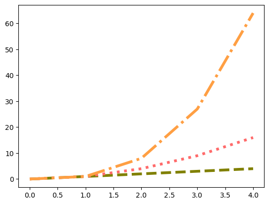

plt.plot(nums, nums, color="olive", marker="*", markersize=20, markerfacecolor="#ff9f43")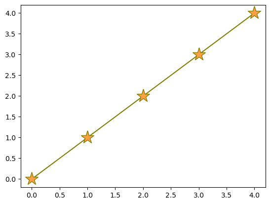

salaries=[55000,65000,72000,90000,115000,150000]
ages = [20,25,30,32,40,45]
plt.plot(ages, salaries)
plt.title("Company Salaries")
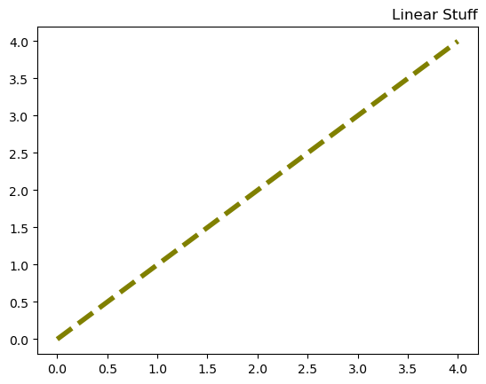
plt.figure()
plt.plot(nums, nums, color="olive", linewidth=4, linestyle="dashed")
plt.title("Linear Stuff", loc="right")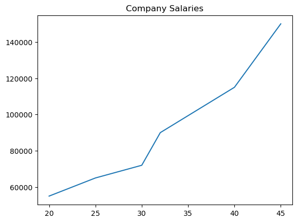

salaries=[55000,65000,72000,90000,115000,150000]
ages = [20,25,30,32,40,45]
plt.plot(ages, salaries)
plt.title("Company Salaries", fontsize=24, color="olive")
plt.xlabel("Employee Age", labelpad=10)
plt.ylabel("Average Salary", labelpad=10 )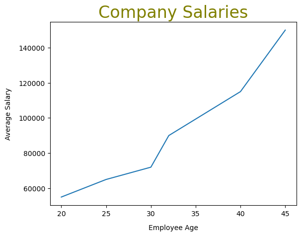

plt.figure(figsize=(8,8))
salaries=[55000,65000,72000,90000,115000,150000]
ages = [20,25,30,32,40,45]
plt.plot(ages, salaries)
plt.title("Company Salaries", fontsize=24, color="olive")
plt.xlabel("Employee Age", labelpad=10)
plt.ylabel("Average Salary", labelpad=10 )
plt.xticks([20,25,30,35,40,45])
plt.yticks([60000,80000,100000, 120000, 140000], labels=["60k", "80k", "100k", "120k","140k"])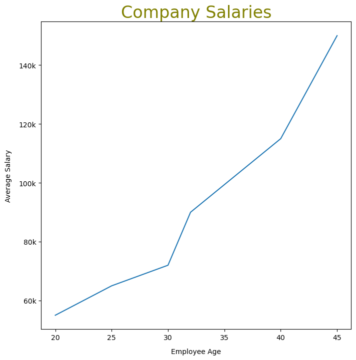

plt.figure(figsize=(8,8))
salaries=[55000,65000,72000,90000,115000,150000]
ages = [20,25,30,32,40,45]
plt.plot(ages, salaries)
plt.xlim(25,40)
plt.ylim(80000, 120000)

(80000.0, 120000.0)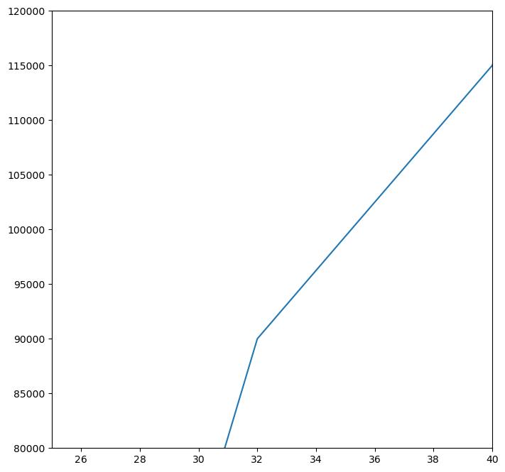

plt.figure(figsize=(5,5))
plt.plot(nums, color="teal", label="x")
plt.plot(nums**2, color="olive", label="x squared")
plt.plot(nums**3, color="purple",label="x cubed")
plt.legend()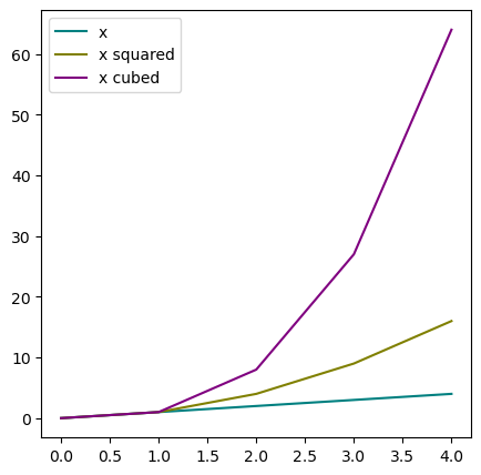

plt.figure(figsize=(5,5))
plt.plot(nums, color="teal", label="x")
plt.plot(nums**2, color="olive", label="x squared")
plt.plot(nums**3, color="purple",label="x cubed")
plt.legend(loc="center left", shadow=True, frameon=True, facecolor="white")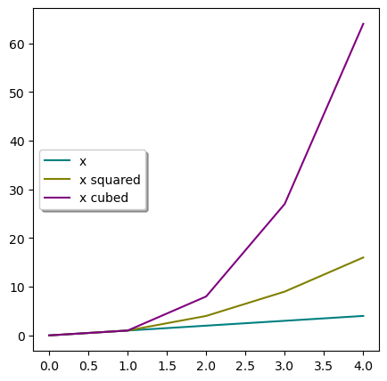

Bar Plots¶

plants = ['Spinach', 'Turnip', 'Rhubarb', 'Broccoli', 'Kale']
died = [10,25,5,30,21]
germinated = [74, 88, 56,69,59]

plt.figure(figsize=(6,6))
plt.bar(plants, germinated, color="orchid")
plt.title("Germination Rates")
plt.ylabel("Number Of Seeldings")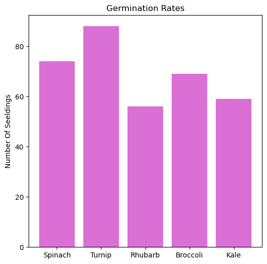

plt.figure(figsize=(6,6))
plt.bar(plants, died, color="red")
plt.title("Failure Rates")
plt.ylabel("Number Of Dead Seedling")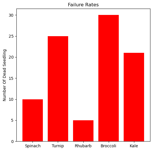

plt.figure(figsize=(6,6))
plt.bar(plants, died, color="#3498db")
plt.bar(plants, germinated, width=0.4, color="#2ecc71", align="edge")

<BarContainer object of 5 artists>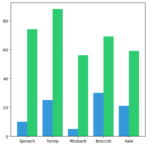

plt.figure(figsize=(6,6))
plt.bar(plants, died, color="#3498db", bottom=germinated )
plt.bar(plants, germinated, color="#2ecc71")

<BarContainer object of 5 artists>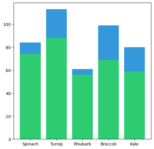

plt.figure(figsize=(6,6))
plt.bar(plants, died, color="#3498db", bottom=germinated,label="Failed Seedlings")
plt.bar(plants, germinated, color="#2ecc71", label="Germinated Seedlings")
plt.legend(shadow=True, frameon=True, facecolor="white")
plt.title("Greenhouse Seedlings")
plt.show()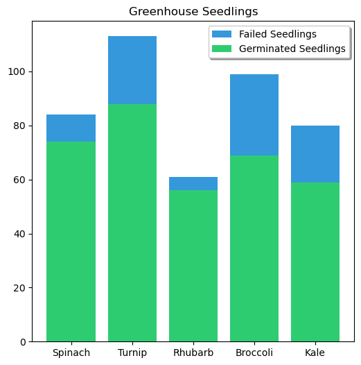

plt.figure(figsize=(6,6))
plt.barh(plants, germinated, color="#2ecc71")

<BarContainer object of 5 artists>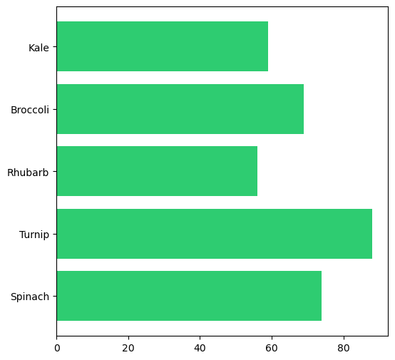

Histograms¶

plt.hist([1,1,2,3,3,3,3,3,4,4,4,5,1,2,1,2,1,2,3,4])

(array([5., 0., 4., 0., 0., 6., 0., 4., 0., 1.]),
 array([1. , 1.4, 1.8, 2.2, 2.6, 3. , 3.4, 3.8, 4.2, 4.6, 5. ]),
 <BarContainer object of 10 artists>)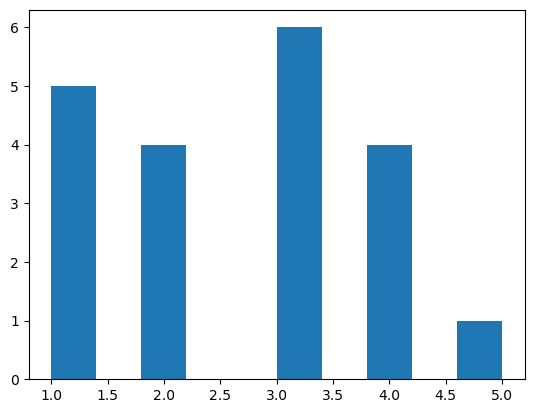

nums = np.random.randn(100)
plt.hist(nums)

(array([ 4.,  3., 12.,  7., 25., 19., 19.,  6.,  3.,  2.]),
 array([-2.38056732, -1.88677616, -1.392985  , -0.89919384, -0.40540268,
         0.08838849,  0.58217965,  1.07597081,  1.56976197,  2.06355313,
         2.55734429]),
 <BarContainer object of 10 artists>)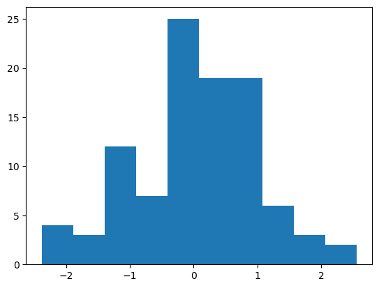

plt.hist(nums, bins=20, color="olive")

(array([ 2.,  2.,  2.,  1.,  9.,  3.,  3.,  4., 11., 14.,  9., 10., 17.,
         2.,  4.,  2.,  2.,  1.,  0.,  2.]),
 array([-2.38056732, -2.13367174, -1.88677616, -1.63988058, -1.392985  ,
        -1.14608942, -0.89919384, -0.65229826, -0.40540268, -0.15850709,
         0.08838849,  0.33528407,  0.58217965,  0.82907523,  1.07597081,
         1.32286639,  1.56976197,  1.81665755,  2.06355313,  2.31044871,
         2.55734429]),
 <BarContainer object of 20 artists>)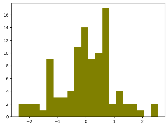

Scatter Plots¶

heights = [137,140,142,145,147,150,152,155,157,160]
f_weights = [28.5,30.8,32.6,34.9,36.4,39,40.8,43.1,44.9,47.2]
m_weights = [34.9,38.1,33.5,35.8,46.7, 42.8,43.1,45.8,50.8,58.9]

plt.scatter(heights, f_weights,  marker="*", label="Female")
plt.scatter(heights, m_weights,marker="d", label="Male")
plt.legend()
plt.xlabel("Height (cm)")
plt.ylabel("Weight (kg)")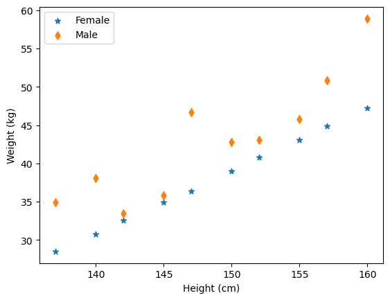

Pie Charts¶

labels = ["Turkey", "Potatoes", "Pumpkin Pie", "Stuffing"]
prices = [25.99,3.24,9.50, 6.99]

plt.pie(prices, labels=labels, autopct="%1.1f%%", shadow=True, explode=(0,0,0.1,0))
plt.show()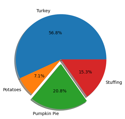

Subplots¶

nums = np.arange(5)
plt.figure(figsize=(10,4))
plt.suptitle("Our First Subplot", fontsize=30)

plt.subplot(1,3,1)
plt.title("X")
plt.plot(nums, nums)

plt.subplot(1,3,2)
plt.plot(nums, nums**2, color="red")
plt.title("X Squared")


plt.subplot(1,3,3)
plt.plot(nums, nums**3, color="yellow")
plt.title("X Cubed")
plt.tight_layout()
plt.show()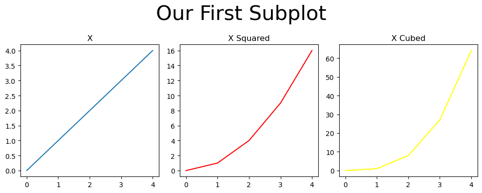

nums = np.arange(5)
plt.figure(figsize=(4,10))
plt.suptitle("Our First Subplot", fontsize=30)

plt.subplot(3,1,1)
plt.title("X")
plt.plot(nums, nums)

plt.subplot(3,1,2)
plt.plot(nums, nums**2, color="red")
plt.title("X Squared")


plt.subplot(3,1,3)
plt.plot(nums, nums**3, color="yellow")
plt.title("X Cubed")
plt.tight_layout()
plt.show()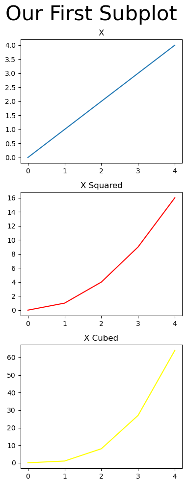

plt.figure(figsize=(8,8))
plt.subplot(2,2,1)
plt.plot(nums)

plt.subplot(2,2,2)
plt.plot(nums)


plt.subplot(2,2,3)
plt.plot(nums)


plt.subplot(2,2,4)
plt.plot(nums)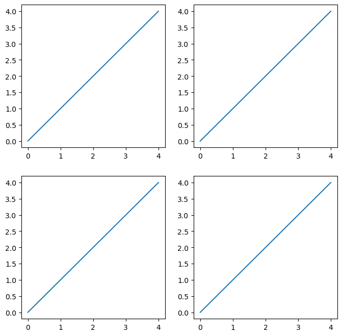

The Object-Oriented Approach¶

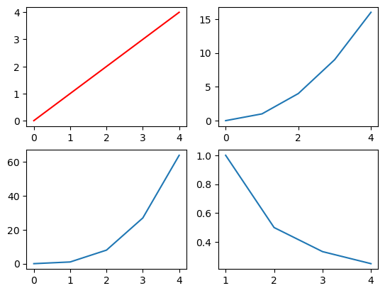
fig, axs = plt.subplots(1,2)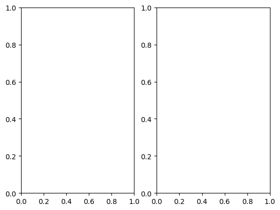

fig, axs = plt.subplots(2,2)
axs[0][0].plot(nums,color="red")
axs[0][1].plot(nums*nums)
axs[1][0].plot(nums**3)
axs[1][1].plot(1/nums)

axs[0][1].set_xticks([0,2,4])

/tmp/ipykernel_11048/2433834221.py:5: RuntimeWarning: divide by zero encountered in divide
  axs[1][1].plot(1/nums)

fig, ax = plt.subplots()
ax.plot(nums)
ax.plot(nums*nums)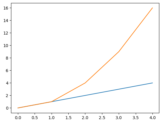

3D Plots¶

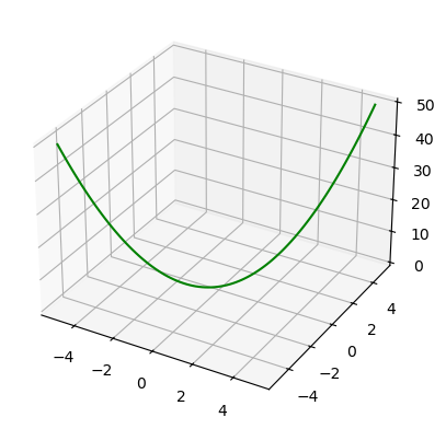
# For 3D plots, let's consider some equations
x = np.linspace(-5, 5, 100)
y = np.linspace(-5, 5, 100)
z = x**2 + y**2

ax = plt.figure().add_subplot(projection='3d')
ax.plot(x, y, z, 'green')

[<mpl_toolkits.mplot3d.art3d.Line3D at 0x7f17616c9090>]